We’ll create linear regression model that predicts price of automobile based on different variables such as make and technical specifications.
Pre-requisite
We’ll use Azure Machine Learning Studio to develop and iterate on simple predictive analytics experiment.
Enter Machine Learning Studio http://studio.azureml.net and click Get started button. We can choose either Guest Access or log in with our Microsoft account.
Machine Learning Studio experiment consists of dragging components to canvas and connecting them in order to create a model, train the model and score and test the model. Experiment uses predictive modelling techniques in form of Machine Learning Studio modules that ingest data, train a model against it and apply model to new data. We can also add modules to pre-process data and select features, split data into training and test sets and evaluate or cross-validate the quality of our model.
Five steps to create experiment
We’ll follow five basic steps to build experiment in Machine Learning Studio in order to create, train and score our model:
- Create model
o Step 1 : Get data
o Step 2 : Pre-process data
o Step 3 : Define features
- Train model
o Step 4 : Choose and apply learning algorithm
- Score and test model
o Step 5 : Predict new automobile prices
Step 1: Get data
There are number of sample datasets included with Machine Learning Studio that we can choose from and we can import data from many sources. For this example, we will use the included sample dataset, Automobile price data (Raw). This dataset includes entries for number of individual automobiles, including information such as make, model, technical specifications and price.
1) Select Blank Experiment. Select default experiment name at the top of canvas and rename it to something meaningful.

2) To left of experiment canvas is palette of datasets and modules. Type automobile in Search box at top of this palette to find dataset labelled Automobile price data (Raw).
3) Drag dataset to experiment canvas.
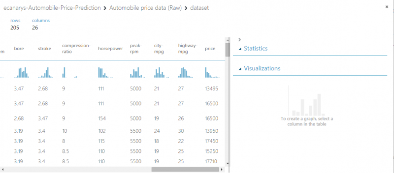
To see what this data looks like, click output port at bottom of automobile dataset and then select Visualize. The variables in the dataset appear as columns and each instance of automobile appears as row. Far-right column is target variable we’re going to try to predict.
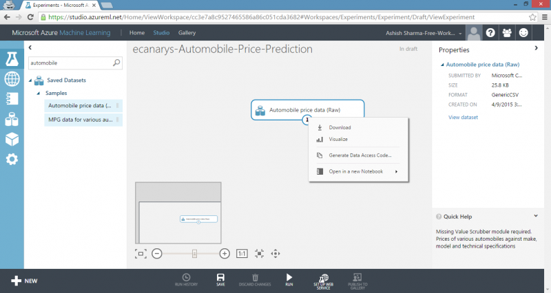
Close the visualization window by clicking the x in upper-right corner.
Step 2: Pre-process data
A dataset usually requires some pre-processing before it can be analysed. We might have noticed missing values present in columns of various rows. These missing values need to be cleaned so model can analyse data correctly. In our case, we’ll remove any rows that have missing values. Also, normalized-losses column has a large proportion of missing values, so we’ll exclude that column from model altogether.
TIP: Cleaning the missing values from input data is pre-requisite for using most of the modules.
First we’ll remove normalized-losses column and then we’ll remove any row that has missing data.
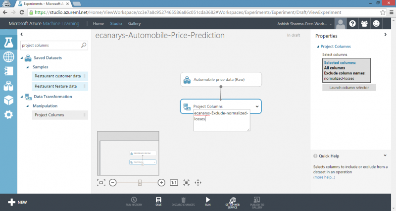
1) Type project columns in Search box at top of module palette to find Project Columns module, then drag it to experiment canvas and connect it to output port of Automobile price data (Raw) dataset. This module allows us to select which columns of data we want to include or exclude in model.
2) Select Project Columns module and click Launch column selector in Properties pane.

- Make sure All columns is selected in filter drop-down list, Begin With. This directs Project Columns to pass through all the columns.
- In next row, select Exclude and column names and then click inside text box. A list of columns is displayed. Select normalized-losses and it will be added to text box.

- Click check mark button to close column selector.

The properties pane for Project Columns indicates that it will pass through all columns from the dataset except normalized-losses.
TIP: We can add a comment to module by double-clicking module and entering text. This can help us to see at glance what module is doing in our experiment. In this case, double-click the Project Columns module and type the comment.
3) Drag Clean Missing Data module to experiment canvas and connect it to Project Columns module. In Properties pane, select Remove entire row under Cleaning mode to clean data by removing rows that have missing values. Double-click module and type comment.


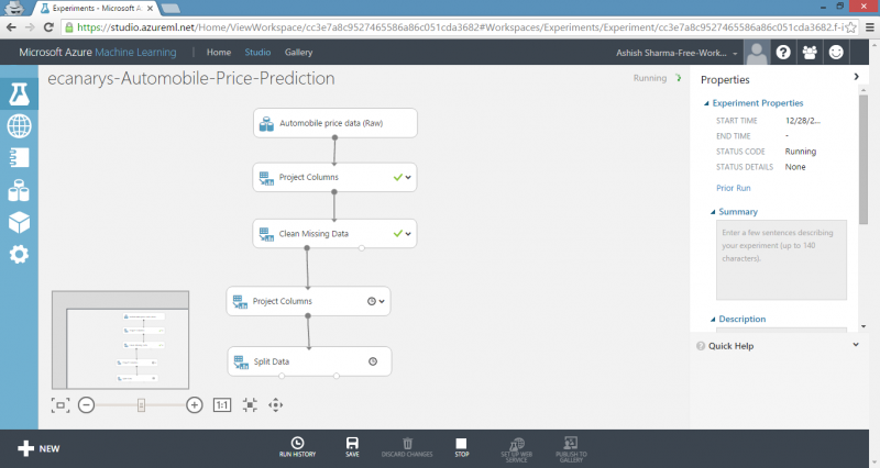
4) Run experiment by clicking RUN under experiment canvas.

When experiment is finished, all modules have green check mark to indicate that they finished successfully. Notice also the Finished running status in upper-right corner.
All we have done in experiment to this point is clean data. If we want to view cleaned dataset, click left output port of the Clean Missing Data module and select Visualize. Notice that normalized-losses column is no longer included and there are no missing values.

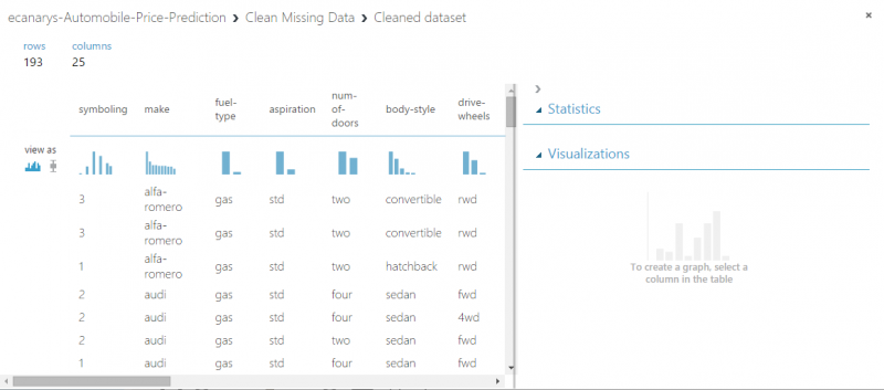
Now that data is clean, we’re ready to specify what features we’re going to use in predictive model.
Step 3: Define features
In machine learning, features are individual measurable properties of something we’re interested in. In our dataset, each row represents one automobile and each column is feature of that automobile. Finding good set of features for creating a predictive model requires experimentation and knowledge about problem we want to solve. Some features are better for predicting target than others. Also, some features have strong correlation with other features, so they will not add much new information to model and they can be removed.
Let’s build model that uses subset of features in our dataset. We can come back and select different features, run experiment again and see if we get better results. As first guess, we’ll select following features with the Project Columns module. Note that for training model, we need to include price value that we’re going to predict.
1) Drag another Project Columns module to experiment canvas and connect it to left output port of the Clean Missing Data module. Double-click module and type comment.
2) Click Launch column selector in Properties pane.

3) In column selector, select No columns for Begin With and then select Include and column names in filter row. Enter our list of column names. This directs module to pass through only columns that we specify.
TIP: Because we’ve run experiment, column definitions for our data have passed from the original dataset through the Clean Missing Data module. When we connect Project Columns to Clean Missing Data, Project Columns module becomes aware of column definitions in our data. When we click the column names box, list of columns is displayed and we can select the columns that we want to add to list.
4) Click check mark button.

This produces dataset that will be used in learning algorithm in next steps. Later, we can return and try again with different selection of features.
Step 4: Choose and apply learning algorithm
Now that data is ready, constructing a predictive model consists of training and testing. We’ll use our data to train model and then test model to see how close it’s able to predict prices.
Classification and regression are two types of supervised machine learning techniques. Classification is used to make prediction from a defined set of values, such as a colour. Regression is used to make a prediction from a continuous set of values, such as a person’s age.
We want to predict price of automobile, which can be any value, so we’ll use a regression model. For this example, we’ll train a simple linear regression model and in next step, we’ll test it.
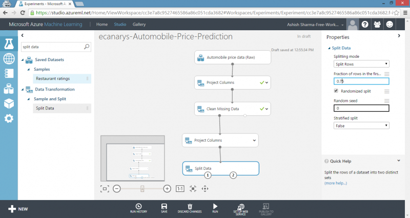
1) We can use our data for both training and testing by splitting it into separate training and testing sets. Select and drag Split Data module to experiment canvas and connect it to output of last Project Columns module. Set Fraction of rows in the first output dataset to 0.75. This way, we’ll use 75 percent of the data to train the model, and hold back 25 percent for testing.
TIP: By changing Random seed parameter, we can produce different random samples for training and testing. This parameter controls the seeding of pseudo-random number generator.
2) Run the experiment. This allows Project Columns and Split Data modules to pass column definitions to the modules we’ll be adding next.

3) To select learning algorithm, expand Machine Learning category in module palette to left of canvas and then expand Initialize Model. This displays several categories of modules that can be used to initialize machine learning algorithms.
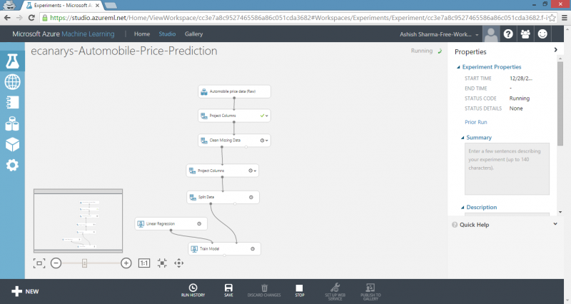
For this experiment, select the Linear Regression module under Regression category and drag it to experiment canvas.
4) Find and drag Train Model module to experiment canvas. Connect left input port to output of Linear Regression module. Connect right input port to training data output of Split Data module.
5) Select the Train Model module, click Launch column selector in Properties pane and then select price column. This is value that our model is going to predict.


6) Run experiment.


The result is trained regression model that can be used to score new samples to make predictions.
Step 5: Predict new automobile prices
Now that we’ve trained model using 75 percent of our data, we can use it to score the other 25 percent of data to see how well our model functions.
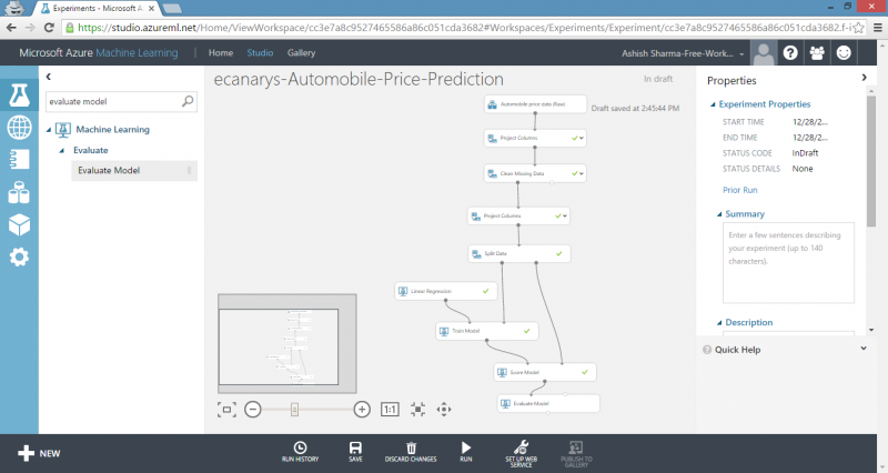
1) Find and drag Score Model module to experiment canvas and connect the left input port to output of the Train Model module. Connect right input port to test data output of Split Data module.
2) To run the experiment and view output from Score Model module, click output port and then select Visualize. Output shows predicted values for price and known values from test data.


3) Finally, to test quality of results, select and drag the Evaluate Model module to experiment canvas and connect left input port to the output of Score Model module.
4) Run experiment.

To view output from Evaluate Model module, click output port and then select Visualize. Following statistics are shown for our model:

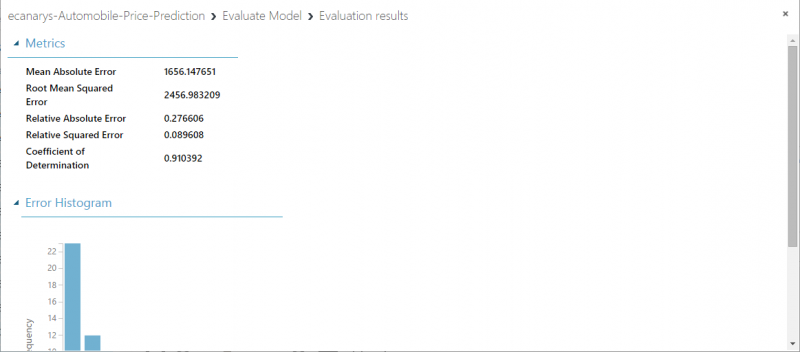
- Mean Absolute Error: The average of absolute errors.
- Root Mean Squared Error: The square root of average of squared errors of predictions made on test dataset.
- Relative Absolute Error: The average of absolute errors relative to absolute difference between actual values and average of all actual values.
- Relative Squared Error: The average of squared errors relative to squared difference between actual values and average of all actual values.
- Coefficient of Determination: Also known as R squared value, this is a statistical metric indicating how well model fits data.
For each of error statistics, smaller is better. A smaller value indicates that predictions more closely match actual values. For Coefficient of Determination, closer its value is to one, better predictions.